Background & Motivation
According to the World Health Organization, road traffic injuries are the leading cause of death for persons aged 5-29 years. While improvements in automobile safety have significantly reduced the dangers of driving, more than 32,000 people are killed and, 2 million are injured each year from motor vehicle crashes in the US alone each year according to the CDC.
As a resident in Denver, I was curious about how safe the roads are that I used to commute by bike each day. I was curious to see if accidents are becoming more frequent over time (possibly due to the population growth in this city), where accidents most frequently occur, and what factors may contribute to or are at least correlated with accidents in this city.
Data
The Denver Open Data Catalog has a dataset that includes motor vehicle crashes reported to the Denver Police Department that occurred within the City and County of Denver and during the previous five calendar years and resulted in at least one thousand dollars in damage, an injury, a fatality, or a drug/alcohol involvement.
The dataset records more than 156,000 traffic incidents. Most of the recorded incidents include information such as the geographic location of the accident, road conditions, human factors that may have contributed to the accident, and any injuries or fatalities that resulted from the accident.
Exploratory Data Analysis
When Accidents Occur
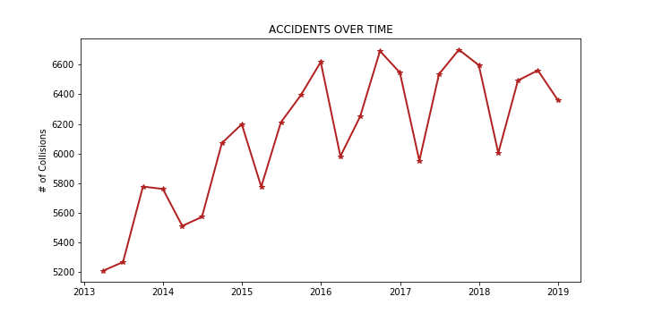
After importing and cleaning my data using pandas, one of my first goals was to determine whether accidents are becoming more frequent. To answer this, I plotted the quarterly total number of crashes from the beginning of 2013 to the end of 2018. There appears to be an increase in the number of accidents year over year, which should be expected in a city which has seen significant population growth. What was surprising, was that there appeared to be a significant seasonality component to the number of accidents, with Q1 of each year marking a considerable decrease in the overall rate of accidents each year.
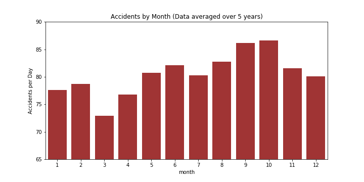
To explore this seasonality component further, I decided to look at the monthly averages over the past five years. Since some months are longer than others, and some years are leap years, I normalized the data to determine the average number of recorded accidents per day in each month of the year. The accident rate appears to increase from March through October and then decrease from October through March of the following year. If I had to guess I would have said that accidents would be most frequent between January and March when snow and ice may contribute to accidents, but the data clearly shows that this is not the case.
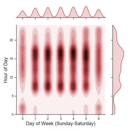
While the seasonality aspect was surprising, I expected to see a positive correlation between commuting times and the number of accidents. The following kernel density estimation (KDE) joint-plot confirms this expectation and reveals that weekdays are particularly bad for traffic accidents between 7-8am and 3-5pm. On the weekends there is also an uptick in the number of accidents that occur during the nighttime hours.
Top Human Contributing Factors
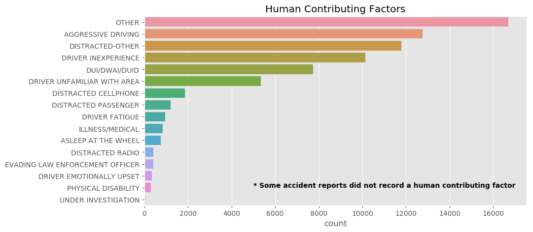
Accident reports sometimes list a human contributing factor. Presumably, this field on the accident report is entered at the reporting Officer’s discretion. It seems likely that there are many cases where these factors are misidentified or not recorded. Since police officers are only working from limited knowledge, this is expected. Nevertheless, this information still reveals some interesting data.
For example, it is interesting that “driver inexperience” is so frequently provided as a contributing factor. I had also expected cell-phone usage to be a more common contributing factor, but it seems likely that many drivers would not volunteer this information and that some accidents resulting from cell-phone use may be grouped under “Distracted-other.”
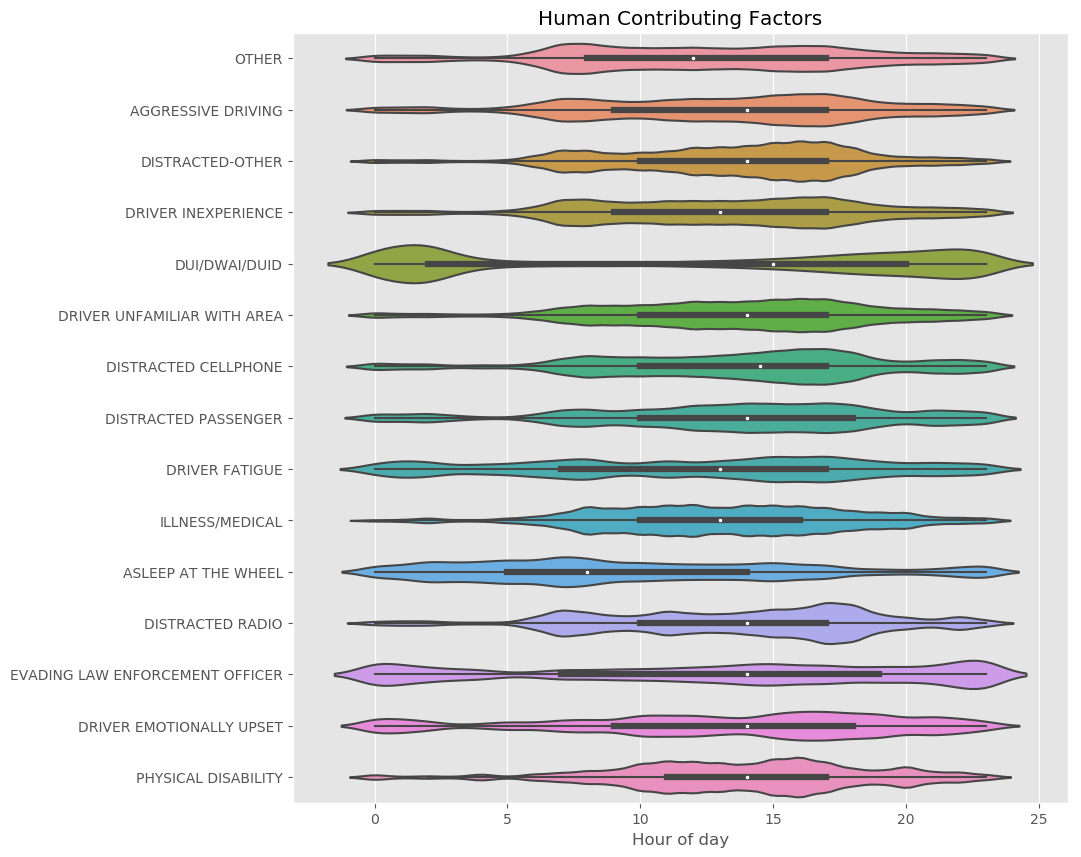
The following violin plots provide some insight into what time of day these contributing factors are likely to be at play. Violin plots are similar to box plots (the inner bar and white dot are indicative of the 25th, 50th, and 75th percentiles), but the ‘thickness of the plot is a kernel density estimation of the distribution. As might be expected, accidents with “DUI,” “Driver fatigue,” “Asleep at the wheel,” “Driver emotionally upset” listed as contributing factors frequently occur during the nighttime hours.
Where do the most Accidents Occur?
Grouping by the “Address” field, I was able to identify the most common accident locations. As can be seen in the table below,the most common places for accidents to occur are onramps or off ramps to the I-25 and I-70 freeways.
| LOCACTION | Count |
|---|---|
| I25 HWYNB / W 6TH AVE | 972 |
| I70 HWYEB / N HAVANA ST | 603 |
| I25 HWYNB / W ALAMEDA AVE | 572 |
| I70 HWYEB / N PEORIA ST | 496 |
| W 6TH AVE / N FEDERAL BLVD | 493 |
| I25 HWYSB / 20TH ST | 476 |
| I25 HWYNB / 20TH ST | 423 |
| I25 HWYNB / E HAMPDEN AVE | 409 |
| I25 HWYSB / W 6TH AVE | 392 |
| I25 HWYNB / W 23RD AVE | 373 |
| I70 HWYEB / N NORTHFIELD QUEBEC ST | 363 |
| I25 HWYSB / W ALAMEDA AVE | 330 |
| I25 HWYNB / W COLFAX AVE | 327 |
| 8400 PENA BLVD | 325 |
| I70 HWYEB / N CENTRAL PARK BLVD | 304 |
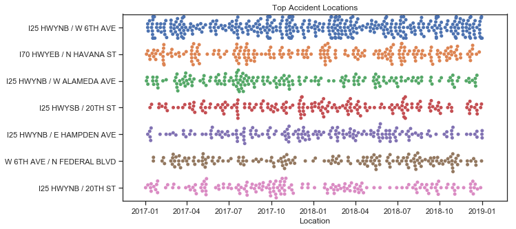
The following plot considers the top 7 locations and plots each accident at the location as a dot over a two year period. There appear to be days, or in some cases weeks, in which these locations may have significantly more or fewer accidents. In some cases, these time periods seem to align between locations, which might be indicative of a contributing factor such as bad weather.
Mapping Accidents
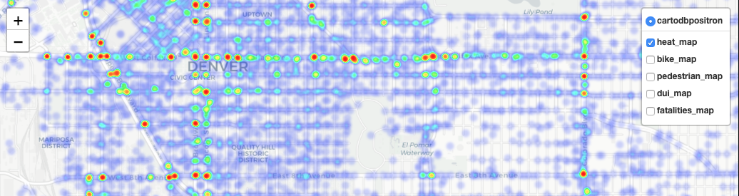
The above insights are interesting, but one thing I really wanted to be able to do was plot data interactively on a map. I did this using folium, which allowed me to create the interactive map linked below.
Please note the interactive layers which can be toggled on and off:
- heat_map - A heat map of all the accidents in the dataset. For the folium heatmap parameters, I used a radius of 5 pixels and a blur effect of 3 and a max intensity of 60.
- bike_map - All accidents involving a cyclist.
- pedestrian_map - All accidents involving a pedestrian.
- dui_map - All accidents where a DUI was listed as a contributing factor
- fatalities_map - All accidents resulting in a fatality.
The html file is also located in the images/ folder of this repo and can be downloaded and run from your local machine.